Second chapter of my study series on Grokking Algorithms by Aditya Y. Bhargava.

• Chapter 1 - Introduction and Binary Search
• Chapter 2 - Arrays, Linked Lists and Selection Sort 📍 you are here
• Chapter 3 - Recursion

I hope you enjoyed the structure from chapter 1 I’ll be keeping the same vibe here. If you have any exercise suggestions or improvements for the explanation, let me know! I’d love the feedback 🫂💕

In chapter 2, the author dives deeper into two fundamental concepts: data structures (like arrays and linked lists) and algorithm efficiency (Big O notation). To illustrate this, he introduces the selection sort algorithm.

Arrays and Linked Lists

Before talking about sorting, it’s important to understand how data can be stored in memory. 👀

The author brings an analogy that makes everything muuuch easier to understand. The idea goes something like this:

Imagine you’re going to a concert and need to leave your things at the coat check (I didn’t even know that was a thing 🤔). Only a few slots are available and you can store one item per slot. You drop your stuff off, close up, and you’re ready to enjoy the show.

Computer memory works a lot like this. The computer is like a huge set of slots, and each slot has an address. Every time you store an item in memory, the computer gives you an address to put it in.

Now, if you want to store multiple items, there are two main ways to do it: arrays and linked lists.

Arrays

• Contiguous blocks of memory each slot is right next to the other.
• Each element can be accessed directly by its index, which makes reading fast.
  • This means the lookup-by-position operation is O(1) constant time.

arr = [10, 20, 30]
print(arr[1])  # direct access to 20

• The downside of arrays is that if you want to add one more item and the next slot is taken, the computer has to find a bigger block of memory and move all existing items there.
• So adding items to an array can be very slow.
• Deleting an element is just as costly all following elements need to be shifted.

Linked Lists

• Items can be stored anywhere in memory.
• Each item stores the address of the next item in the list.
• Kind of like a treasure hunt each clue tells you where the next one is.
• Adding an item is simple: just put it anywhere in memory and update the previous item’s pointer.
• Deleting is just as easy: just change the previous item’s pointer to skip over the one you want to remove.
• The downside of linked lists is that to access a specific element (say, the last one), you can’t jump straight to it you have to walk through the list one item at a time.

class Node:
    def __init__(self, value):
        self.value = value
        self.next = None

a = Node(10)
b = Node(20)
a.next = b

# Traversing
n = a
while n:
    print(n.value)
    n = n.next

Breaking down the code above: 1. I create the Node class, which stores a value (value) and a pointer to the next node (next). 2. I create two nodes: a with value 10 and b with value 20. 3. I link a to b with a.next = b. 4. I traverse the list with while n:, printing n.value until I reach the end (None).

Output:

10
20

I don’t know about you, but understanding the difference between arrays and linked lists was a real lightbulb moment for me. Since I learned Python first, I kind of used these structures on autopilot… 🥲 It might seem obvious or even unnecessary after all, we deal with arrays and lists all the time but it was incredible to finally understand why things work the way they do. My brain finally started connecting the dots and seeing the logic behind it all. I was kind of like:

Here are the running times for the most common operations on arrays and linked lists:

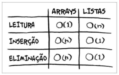
I think it’s important to have this table handy to reinforce Big O notation and help everyone understand the impact of our choices in different situations.

A more explicit breakdown:

• Reading:

  • Array → O(1): In an array, each position has a fixed address in memory. So if you want the 5th element, the computer goes straight to it super fast, constant time.

  • Linked List → O(n): In a linked list, each element only knows who comes next. So to find the 5th element, you have to start from the 1st, then the 2nd, then the 3rd… all the way to the 5th. The bigger the list, the longer it takes.

• Insertion:

  • Array → O(n): If the array is full and you want to insert a new item in the middle, you have to “push” all other elements one position forward. That can take a while.

  • Linked List → O(1): If you already know the position, inserting into a linked list is quick just change who points to whom, and you’re done.

• Deletion:

  • Array → O(n): If you remove an item from the middle of an array, you have to “pull” all the elements after it one position back to close the gap.

  • Linked List → O(1): Just like insertion, you just update the pointers to skip the item you want to remove. Nothing else needs to move.

Selection Sort

The author presents the Selection Sort algorithm simple to implement, but not very efficient. Understanding the difference between arrays and linked lists makes it important to see how the algorithm traverses and manipulates elements.

How it works

1. Find the smallest element in the list
2. Place it in the first position
3. Repeat for the remaining positions until the whole list is sorted

Python implementation:

def find_smallest(arr):
    """
    Finds the index of the smallest element in an array.

    Parameters:
    arr (list): A list of comparable elements.

    Returns:
    int: Index of the smallest element found.
    """
    smallest = arr[0]
    smallest_index = 0
    for i in range(1, len(arr)):
        if arr[i] < smallest:
            smallest = arr[i]
            smallest_index = i
    return smallest_index

def selection_sort(arr):
    """
    Sorts a list using the selection sort algorithm.

    The function creates a new list by removing the smallest element
    from the original list at each iteration and appending it to the sorted list.

    Parameters:
    arr (list): A list of numbers to sort.

    Returns:
    list: A new list sorted in ascending order.
    """
    new_arr = []
    for i in range(len(arr)):
        smallest = find_smallest(arr)
        new_arr.append(arr.pop(smallest))
    return new_arr

print(selection_sort([5, 3, 6, 2, 10]))  # Output: [2, 3, 5, 6, 10]

Complexity and Big O

• Selection sort needs to traverse all elements multiple times.
• For n elements, it performs roughly n × n operations.
• This means its performance is O(n²).

This is a classic example of how different algorithms can solve the same problem with different efficiencies, highlighting the importance of choosing the right algorithm based on the size and structure of your data.

Fun facts

• Lists in Python are actually arrays.
• The append method (adding to the end) is considered O(1) on average. That’s because adding to the end is cheap: just place the item in the next available slot.
• The “expensive” part shows up with operations like insert or remove in the middle. Those require shifting all following elements, which can be O(n).
• A good way to visualize: think of a stack of plates. Putting or taking a plate from the top (append and pop) is easy. But if you want to insert or remove one from the middle (insert or remove), you have to move all the plates above it first.

Recommended exercises 👩🏻‍💻💞

Here are some practical challenges to reinforce what you learned:

LeetCode

• Two Sum classic array problem
• Best Time to Buy and Sell Stock traversing an array with time analysis
• Merge Sorted Array sorted list manipulation

Exercism

• Isogram traverses strings/arrays checking for duplicates

And that wraps up chapter 2! I hope it was useful and easy to read 💁🏻‍♀️✨

Compartilhar: