Start of a study series on the book Grokking Algorithms by Aditya Y. Bhargava.
- Chapter 1 - Introduction and Binary Search 📍 you are here
- Chapter 2 - Arrays, Linked Lists and Selection Sort
- Chapter 3 - Recursion
This book was recommended by a friend, Ana Paula Mendes, and I had no idea how much I’d love it. The writing is light, clear, and very accessible. If you, like me, have a hard time staying consistent with technical reading, this book is a gem easy to understand, great for learning or revisiting concepts.
It presents computer science ideas that show up in our everyday lives, often without us even noticing.
One of the things I love most about this book is how the author teaches always through examples. Instead of overwhelming you with symbols and formulas, he wants you to visualize the concepts. He believes and I agree that we learn better when we can connect new content to something we already know. And examples are the best way to do that.
And the best part? He literally draws 🤩! You know when someone says “do you want me to draw it for you?” I always say “yes, please!” and he actually does. It’s wonderful ✨.
You can feel that everything was thought through carefully: the content, the illustrated examples, and the recap at the end of each chapter.
With that intro out of the way, let’s see what chapter 1 is all about!

Binary search in a nutshell
Imagine a phone book with 1 million names. Going page by page would be a nightmare, right? Now, what if I told you that you can find any name in at most 20 tries? 👀
The trick is simple: at each step, you eliminate half the options. Start with the element right in the middle of the sequence. In a phone book, that would be opening it right in the middle. In a list of 10 items, that’s picking the 5th one. Now compare that middle item with what you’re looking for: if they match congrats, you found it! If the middle item is GREATER than what you’re looking for (think alphabetical order for names), the item must be in the first half. Otherwise, it’s in the second half. This way, you cut the list in half with just one comparison. Then you take the selected half and repeat the same strategy.
Note: This only works if the list is sorted!
And the coolest part? Even if the list doubles in size, you only need one more step to find the result. 🤓
Example: Let’s use a smaller list of 128 names and calculate the maximum number of steps to find a specific one. Then we double the list and see it only adds one more step:
def max_steps(n):
    steps = 0
    while n > 1:
        n //= 2
        steps += 1
    return steps

print(max_steps(128))    # 7
print(max_steps(128*2))  # 8
Important note: with a physical phone book, we already know to jump almost directly to the right letter which is more like how a hashmap (or Python dict) works, finding an item in constant time. But in a computer, when you only have a sorted list (like [1, 3, 5, 7, 9, 11, 13]), there’s no such “magic jump” that’s where binary search helps, cutting the list in half systematically until it finds the item (or confirms it’s not there).
Pretty cool, right? That’s computer science!! 💁♀️✨
Basic binary search examples
Think of a number between 1 and 100. You can guess it in at most 7 tries:
My first question: “Is it 50?”
- If you say “higher”, I know it’s between 51 and 100
- If you say “lower”, it’s between 1 and 49
Second question: Let’s say it’s higher than 50. “Is it 75?” (midpoint between 51 and 100)
- Higher? It’s between 76 and 100
- Lower? It’s between 51 and 74
And so on always cutting the possibilities in half.
Let’s see how it scales with larger numbers:
| Items in list | Linear search (tries) | Binary search (tries) |
|---|---|---|
| 1,000 | up to 1,000 | up to 10 |
| 1,000,000 | up to 1,000,000 | up to 20 |
Yes 20 tries to find something among 1 million options! 🚀
This “miracle” happens because of a concept called logarithms and I’ll show you why in just a moment.
Now that you understand binary search, let’s look at three things that go hand in hand with it: logarithms, running time, and Big O notation.
Here’s a quick summary of each, broken down the way that made sense to me. If something gets confusing, no worries just check the book, it’s great 🫂💖
Logarithms
The maximum number of tries in binary search is given by log₂(n) the base-2 logarithm of n.
If the name sounds scary, think of it this way:
log₂(n) is how many times you need to divide n by 2 until you reach 1
Example:
- log₂(128) = 7 7 halving steps until 1 item remains
- log₂(256) = 8 just one more step, even though the list doubled
The base “2” comes from the fact that at each step we cut the list in half.
Running time
Whenever we talk about an algorithm, it’s important to think about running time how much effort (or how many steps) it needs to reach a result.
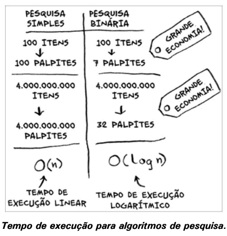
With linear search (simple search), we check item by item:
- List with 100 numbers → up to 100 tries
- List with 4 billion numbers → up to 4 billion tries
The running time grows in direct proportion to the list size. We call this linear time.
Binary search is a different story:
- List with 100 numbers → at most 7 tries
- List with 4 billion → at most 32 tries
This happens because binary search cuts the possibilities in half at every step. This type of growth is called logarithmic time.
Big O Notation
Big O notation is a way to measure the efficiency of an algorithm showing how running time grows as the input size increases.
- O(log n) logarithmic time (e.g. binary search)
- O(n) linear time (e.g. simple search)
- O(n * log n) a fast sorting algorithm, like quicksort (Chapter 4)
- O(n²) a slower sorting algorithm, like selection sort (Chapter 2)
- O(n!) an extremely slow algorithm, like the traveling salesperson (Chapter 1)
The book illustrates this in a very visual and intuitive way: grows linearly, grows in log, grows a lot, grows slowly… and so on.
Now that we’ve seen how binary search works, it’s worth noting that it’s not just for phone books it shows up in many real-life situations:
- Search systems (Google, WhatsApp, Spotify): under the hood, they use variations of binary search on sorted lists or indexes.
- Data filtering: quickly finding a specific record in large spreadsheets or databases.
- Debugging: reducing the problem space by half at each test to find where the bug is.
Note: for binary search to work, the data must be sorted.
Quick practice?
Here’s a sorted list of numbers: [2, 4, 6, 8, 10, 12, 14, 16, 18, 20, 22, 24, 26, 28, 30, 32]
Try to find the number 22 in two ways:
- Linear search: go one by one starting from 2.
- Binary search: start in the middle, eliminate half at each step.
Compare how many steps each method took!
Fun facts
- Git has a feature called
git bisectthat uses binary search to help developers find bugs - If the item we’re looking for is the first in the list, that’s the best case for linear search and the worst case for binary search
- The
sortedcontainersimplementation uses binary search (via thebisectmodule) see here
Recommended exercises 👩🏻💻💞
Here are some practical challenges to reinforce what you learned:
LeetCode
- Binary Search straightforward implementation.
- Search Insert Position variation to find where to insert a number.
- First Bad Version binary search applied to an API.
Exercism
- Binary Search (Python Track) implementation and tests.
Tip: try to solve the problem before looking at any solution, then compare your approach with optimized implementations.
And so begins my study roadmap: each chapter of the book comes with exercises to reinforce the content.